4.14. Custom functionals 1
This example gives an example of how eminus can be extended at runtime, e.g., by using custom functionals. Also, this example outlines how one can parameterize their own LDA functional.
import matplotlib.pyplot as plt
import numpy as np
from scipy.optimize import curve_fit

import eminus.xc
from eminus import Atoms, SCF
from eminus.units import ry2ha
Start with a normal SCF calculation for helium with the original LDA Chachiyo functional
atoms = Atoms("He", (0, 0, 0), ecut=10, verbose=0)
scf = SCF(atoms, xc="lda,chachiyo")
scf.run()
print(f"Energies with the Chachiyo functional:\n{scf.energies}")
Define arrays for the Quantum Monte Carlo (QMC) results from Ceperley and Alder for the homogeneous electron gas
The values are the paramagnetic correlation energies from Tab. 5 in Can. J. Phys. 58, 1200
rs = np.array([2, 5, 10, 20, 50, 100])
# Convert from -mRy to Hartree
ecp = -ry2ha(np.array([90.2, 56.3, 37.22, 23.00, 11.40, 6.379])) / 1000
Define the original Chachiyo functional parameters
The parameters are derived such that the functional recovers the values in Phys. Rev. B 84, 033103 for the high-density limit
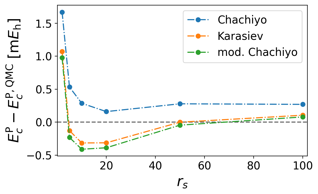
Karasiev re-parameterized the functional in J. Chem. Phys. 145, 157101 without the restriction of b=c
Here, c uses the same value as in Chachiyo to preserve the correct high-density limit but b is chosen such that it recovers the exact value for rs=50
We will now build a new custom functional by fitting b over the QMC data set
a = (np.log(2) - 1) / (2 * np.pi**2)
c = 20.4562557
b = c
print(f"\nOriginal parameter:\nb = {b:.7f}")
All functionals in eminus share the same signature and return types
Define a custom spin-paired functional using said signature based on the Chachiyo functional but with the customizable parameter parameter b so we can fit over it
def custom_functional(n, b, **kwargs):
    rs = (3 / (4 * np.pi * n)) ** (1 / 3)  # Wigner-Seitz radius
    ec = a * np.log(1 + b / rs + c / rs**2)  # Exchange energy
    vc = ec + a * (2 * c + b * rs) / (3 * (c + b * rs + b * rs**2))  # Exchange potential
    return ec, np.array([vc]), None
Fit the functional using a wrapper function
We only fit over the energies so the wrapper function only returns the first argument of the functional
The third return value of the function (here None) is only used in GGA functionals
Functionals usually take densities as the input, so convert the Wigner-Seitz radius to a density in the wrapper function
def functional_wrapper(rs, b):
    n = 3 / (4 * np.pi * rs**3)  # Density from Wigner-Seitz radius
    return custom_functional(n, b)[0]
Do the fit over the QMC data
The resulting parameter still recovers the limits of the original functional but can be more accurate in the mid-density regimes
One can see that our fitted value is similar to the one derived by Karasiev with b=21.7392245
fitted_b, _ = curve_fit(functional_wrapper, rs, ecp)
print(f"\nFitted parameter:\nb = {fitted_b[0]:.7f}")
# Fitted parameter:
# b = 21.9469106
Plot the error of the correlation energies compared to the QMC data for Chachiyo, Karasiev, and our functional
Find the plot named correlation_energy_error.png

plt.style.use("../eminus.mplstyle")
plt.figure()
plt.axhline(c="dimgrey", ls="--", marker="")
plt.plot(rs, 1000 * (functional_wrapper(rs, b) - ecp), label="Chachiyo")
plt.plot(rs, 1000 * (functional_wrapper(rs, 21.7392245) - ecp), label="Karasiev")
plt.plot(rs, 1000 * (functional_wrapper(rs, *fitted_b) - ecp), label="mod. Chachiyo")
plt.xlabel(r"$r_s$")
plt.ylabel(r"$E_c^\mathrm{P} - E_c^{\mathrm{P,QMC}}$ [m$E_\mathrm{h}$]")
plt.legend()
plt.savefig("correlation_energy_error.png")
Some modules of eminus have an IMPLEMENTED lookup dictionary for functions that can be extended
These are available in the xc, potentials, and minimizer modules and can be used as seen below
Plug the fitted parameters into the custom functional
eminus.xc.IMPLEMENTED["custom"] = lambda n, **kwargs: custom_functional(n, *fitted_b)
If the signature of the custom functional matches the signature from eminus it is sufficient to write
# eminus.xc.IMPLEMENTED["custom"] = custom_functional
Start an SCF calculation with our custom functional
scf = SCF(atoms, xc="lda,custom")
scf.run()
print(f"\nEnergies with the fitted Chachiyo functional:\n{scf.energies}")
An extension of this example for the spin-polarized case can be found in the next example
Download 14_custom_functionals.py correlation_energy_error.png