4.17. Reduced density gradient
In eminus, most variables field variables can be accessed and are discretized on a grid. Also, gradients are available. This example reduces some plots from the paper J. Chem. Theory Comput. 20, 68.
import matplotlib.pyplot as plt

from eminus import Atoms, SCF
from eminus.tools import get_reduced_gradient
from eminus.units import ang2bohr
Do an RKS calculation for hydrogen with the given bond distance
atoms = Atoms("H2", [[0.0, 0.0, 0.0], [0.0, 0.0, ang2bohr(0.75)]], center=True)
scf = SCF(atoms)
scf.run()
One can even use thermal exchange-correlation functionals using Libxc
One example would be the following, where the temperature parameter of the functional gets modified (in Hartree)
# scf = SCF(atoms, xc=":LDA_XC_GDSMFB")
# print(scf.xc_params_defaults)
# scf.xc_params = {"T": 0.1}
# scf.run()
Calculate the truncated reduced density gradient
s = get_reduced_gradient(scf, eps=1e-5)
Write n and s to CUBE files
One can view them, e.g., with the eminus.extras.view function in a notebook
# scf.write("density.cube", scf.n)
# scf.write("reduced_density_gradient.cube", s)
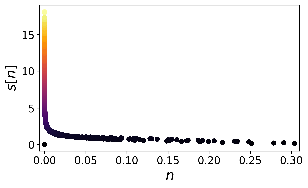
Plot s over n
Compare with figure 2 of the supplemental material
Find the plot named density_finger.png

plt.style.use("../eminus.mplstyle")
plt.figure()
plt.scatter(scf.n, s, c=s)
plt.xlabel("$n$")
plt.ylabel("$s$[$n$]")
plt.savefig("density_finger.png")