4.13. Geometry optimization
This example serves as a minimal example for geometry optimizations by finding the optimal bond distance in the H2 molecule.
import matplotlib.pyplot as plt
import numpy as np
from scipy.optimize import minimize_scalar

from eminus import Atoms, SCF
from eminus.units import bohr2ang, ha2ev
Create lists to save intermediate results of the optimization
distances = []
energies = []
Create a simple cost function for the optimizer
The objective is of course the total energy of the molecule
Displace one hydrogen by a distance d, choose a small ecut for a faster evaluation
def cost(d):
    atoms = Atoms("H2", [[0, 0, 0], [0, 0, d]], ecut=5)
    scf = SCF(atoms, verbose=0)
    etot = scf.run()
    print(f"d={bohr2ang(d):.6f} A    Etot={ha2ev(etot):.6f} eV")
    distances.append(d)
    energies.append(etot)
    return etot
The total energy for an H2 molecule will be saved in the above lists when calling the cost function
cost(0.5)
Since we only optimize one value here, we use the minimize scalar function
We also add bounds since d=0 should be forbidden
When optimizing multiple coordinates one can give a reasonable start configuration instead of giving explicit bounds
res = minimize_scalar(cost, bounds=(0.1, 10))
print(f"Optimized bond length: {bohr2ang(res.x):.6f} A")
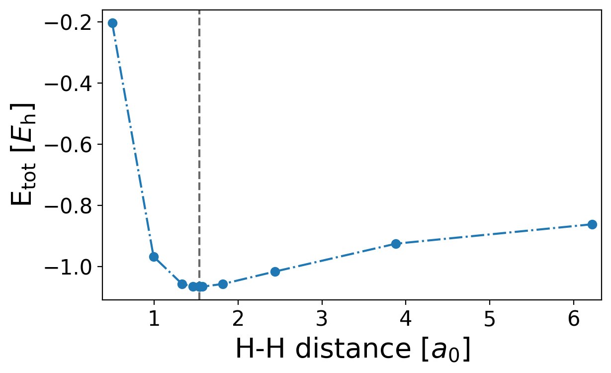
With the saved intermediate H-H distances and the respective energies one can generate a potential energy surface plot
Find the plot named dissociation_energy_h2.png

plt.style.use("../eminus.mplstyle")
sort = np.argsort(distances)
plt.figure()
plt.axvline(res.x, c="dimgrey", ls="--", marker="")
plt.plot(np.array(distances)[sort], np.array(energies)[sort])
plt.xlabel(r"H-H distance [$a_0$]")
plt.ylabel(r"E$_\mathrm{tot}$ [$E_\mathrm{h}$]")
plt.savefig("dissociation_energy_h2.png")
The procedure could also be done, e.g., for optimizing the lattice constant of a germanium solid as seen in example 12
Downloads: 13_geometry_optimization.py dissociation_energy_h2.png