4.15. Custom functionals 2
This example extends the previous example by re-parameterizing the Chachiyo functional for the spin-polarized case.
import matplotlib.pyplot as plt
import numpy as np
from scipy.optimize import curve_fit

from eminus.units import ry2ha
from eminus.xc.lda_c_chachiyo import chachiyo_scaling
Wigner-Seitz radii and the respective densities
rs = np.array([2, 5, 10, 20, 50, 100])
n = 3 / (4 * np.pi * rs**3)
Paramagnetic and ferromagnetic QMC values for the homogeneous electron gas
ecp = -ry2ha(np.array([90.2, 56.3, 37.22, 23.00, 11.40, 6.379])) / 1000
ecf = -ry2ha(np.array([48.0, 31.2, 21.0, 13.55, 7.09, 4.146])) / 1000
Original Chachiyo parameters and our fitted value from the paramagnetic case
b0 = 20.4562557
b1 = 27.4203609
fitted_b0 = 21.9469106
print(f"Original parameter:\nb1 = {b1:.7f}")
Spin-polarized Chachiyo functional with additional fit parameters
We won’t do an extra DFT calculation with this functional, so the function only returns the correlation energies and no potentials
def lda_c_chachiyo_spin(n, zeta, b0, b1):
    a0 = (np.log(2) - 1) / (2 * np.pi**2)
    a1 = (np.log(2) - 1) / (4 * np.pi**2)
    c0 = 20.4562557
    c1 = 27.4203609

    rs = (3 / (4 * np.pi * n)) ** (1 / 3)
    ec0 = a0 * np.log(1 + b0 / rs + c0 / rs**2)
    ec1 = a1 * np.log(1 + b1 / rs + c1 / rs**2)
    return ec0 + (ec1 - ec0) * chachiyo_scaling(zeta)[0]
Again, define a wrapper function for the optimization
In the ferromagnetic case we have a relative spin density of 1 (with 0 we would recover the paramagnetic case)
def functional_wrapper(rs, b1):
    n = 3 / (4 * np.pi * rs**3)
    return lda_c_chachiyo_spin(n, 1, fitted_b0, b1)
Do the fit over the QMC data
One can see that our fitted value is vastly different from the one derived by Karasiev with b1=28.3559732
fitted_b1, _ = curve_fit(functional_wrapper, rs, ecf)
print(f"\nFitted parameter:\nb1 = {fitted_b1[0]:.7f}")
# Fitted parameter:
# b1 = 26.9515208
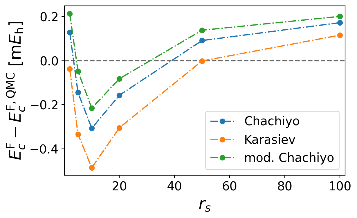
Plot the error of the correlation energies compared to the QMC data for Chachiyo, Karasiev, and our functional
Find the plot named correlation_energy_error_spin.png

plt.style.use("../eminus.mplstyle")
plt.figure()
plt.axhline(c="dimgrey", ls="--", marker="")
plt.plot(rs, 1000 * (lda_c_chachiyo_spin(n, 1, b0, b1) - ecf), label="Chachiyo")
plt.plot(rs, 1000 * (lda_c_chachiyo_spin(n, 1, 21.7392245, 28.3559732) - ecf), label="Karasiev")
plt.plot(rs, 1000 * (lda_c_chachiyo_spin(n, 1, fitted_b0, *fitted_b1) - ecf), label="mod. Chachiyo")
plt.xlabel(r"$r_s$")
plt.ylabel(r"$E_c^\mathrm{F} - E_c^{\mathrm{F,QMC}}$ [m$E_\mathrm{h}$]")
plt.legend()
plt.savefig("correlation_energy_error_spin.png")
Lastly, let us compare the mean absolute errors (MAE) of these functional variants
One could also compare the root mean square error but the result would be obvious since our fit minimizes this error
def mae(data, ref):
    return 1000 * np.sum(np.abs(data - ref)) / len(ref)
Begin with the spin-paired case…
print("\nMAE (spin-paired) [mEh]:")
print(f"Chachiyo: {mae(lda_c_chachiyo_spin(n, 0, b0, b1), ecp):.3f}")
print(f"Karasiev: {mae(lda_c_chachiyo_spin(n, 0, 21.7392245, 28.3559732), ecp):.3f}")
print(f"Modified: {mae(lda_c_chachiyo_spin(n, 0, fitted_b0, *fitted_b1), ecp):.3f}")
# MAE (spin-paired) [mEh]:
# Chachiyo: 0.533
# Karasiev: 0.322
# Modified: 0.355
…and end with the spin-polarized case
print("\nMAE (spin-polarized) [mEh]:")
print(f"Chachiyo: {mae(lda_c_chachiyo_spin(n, 1, b0, b1), ecf):.3f}")
print(f"Karasiev: {mae(lda_c_chachiyo_spin(n, 1, 21.7392245, 28.3559732), ecf):.3f}")
print(f"Modified: {mae(lda_c_chachiyo_spin(n, 1, fitted_b0, *fitted_b1), ecf):.3f}")
# MAE (spin-polarized) [mEh]:
# Chachiyo: 0.167
# Karasiev: 0.213
# Modified: 0.150
One can see that our functional outperforms the original Chachiyo functional in both cases (obviously since we compare to the data we fitted to)
Surprisingly, the parameterization from Karasiev performs a bit better in the paramagnetic case but is worse in the ferromagnetic case
Our functional seems to perform well in both cases
Downloads: 15_custom_functionals_spin.py correlation_energy_error_spin.png