4.17. Reduced density gradient
In eminus, most variables field variables can be accessed and are discretized on a grid. Also, gradients are available. This example reduces some plots from the paper J. Chem. Theory Comput. 20, 68.
import matplotlib.pyplot as plt

from eminus import Atoms, SCF
from eminus import backend as xp
from eminus.tools import get_reduced_gradient
from eminus.units import ang2bohr
Do an RKS calculation for hydrogen with the given bond distance
atoms = Atoms("H2", [[0.0, 0.0, 0.0], [0.0, 0.0, ang2bohr(0.75)]], center=True)
scf = SCF(atoms)
scf.run()
One can even use thermal exchange-correlation functionals
One example would be the following, where the temperature parameter of the functional gets modified (in Hartree)
# scf = SCF(atoms, xc="LDA_XC_GDSMFB")
# print(scf.xc_params_defaults)
# scf.xc_params = {"T": 0.1}
# scf.run()
Calculate the truncated reduced density gradient
s = get_reduced_gradient(scf, eps=1e-5)
Write n and s to CUBE files
One can view them, e.g., with the eminus.extras.view function in a notebook
# scf.write("density.cube", scf.n)
# scf.write("reduced_density_gradient.cube", s)
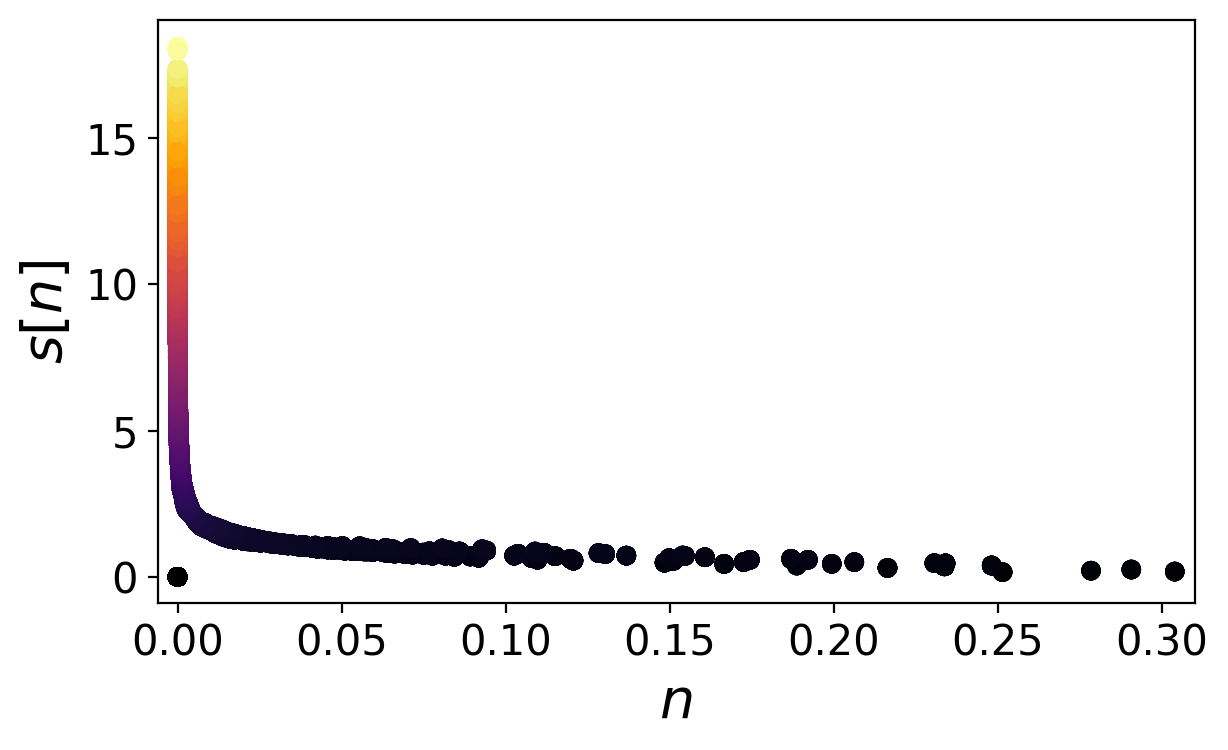
Plot s over n
Compare with figure 2 of the supplemental material
Find the plot named density_finger.png

plt.style.use("../eminus.mplstyle")
plt.figure()
plt.scatter(xp.to_np(scf.n), xp.to_np(s), c=xp.to_np(s))
plt.xlabel("n")
plt.ylabel("s")
plt.savefig("density_finger.png")
Downloads: 17_reduced_density_gradient.py density_finger.png