3. Tutorial
var_mesh package. The code snippets can be executed in a Python shell when going from top to bottom. When looking at specific examples, some previous inputs may be necessary to run them. To run the example separately, the script can be found at the bottom of the section.>>> import var_mesh
3.1. Minimal example
With the goal in mind to optimize meshes for further DFT calculations, a simple example calculation for water can be done. For this, the necessary pyscf and var_mesh modules need to be imported.
>>> from pyscf import dft, gto
>>> from var_mesh import var_mesh
Next, the water mol object can be created, along with the RKS object for the restricted Kohn-Sham SCF calculation.
>>> mol = gto.M(atom='O 0 0 0; H 0 0 0.95691; H 0.95691 0 -0.23987')
>>> mf = dft.RKS(mol)
Calling the function var_mesh() and overwriting the existing Grids object will create the optimized mesh for the calculation, which can be started afterwards.
>>> mf.grids = var_mesh(mf.grids)
Atom grids = {'H': (30, 110), 'O': (60, 302)}
>>> mf.kernel()
converged SCF energy = -74.7350158141935
The output from var_mesh() can be reused for future calculations.
>>> mf.grids.atom_grid = {'H': (30, 110), 'O': (60, 302)}
>>> mf.kernel()
converged SCF energy = -74.7350158141935
The script for this example can be downloaded here.
3.2. Custom grids
Instead of default PySCF grid levels, custom radial or angular grids can be used as well. For this, the parameters rad or ang can be overwritten with dictionaries that have the atom type identifiers as keys, with lists of the respective number of grids as values.
>>> from var_mesh import gen_mesh
>>> gen_mesh.rad = {'H': list(range(10, 100, 15)), 'O': list(range(20, 200, 20))}
>>> print(gen_mesh.rad)
{'H': [10, 25, 40, 55, 70, 85], 'O': [20, 40, 60, 80, 100, 120, 140, 160, 180]}
The angular grids have to follow the Lebedev order. The array ang_grids can be used for this purpose and contains all possible grid numbers.
>>> gen_mesh.ang = {'H': gen_mesh.ang_grids[15:20], 'O': gen_mesh.ang_grids[20:25]}
>>> print(gen_mesh.ang)
{'H': array([350, 434, 590, 770, 974]), 'O': array([1202, 1454, 1730, 2030, 2354])}
Different attributes of the Grids class can also freely be used and will be respected in the optimizations. See the documentation for more details.
>>> mesh = dft.Grids(mol)
>>> mesh.prune = None
Changing the attribute verbose will change the amount of output of the var_mesh() function, with the maximum output at level 6. The error threshold can be changed as well.
>>> mesh.verbose = 5
>>> mesh = var_mesh(mesh, thres=1e-7)
Start coarse grid search.
[1/5] Error = 5.79931e-04
[2/5] Error = 1.44722e-07
[3/5] Error = 2.00122e-08
Error condition met.
Level = 2
Start fine grid search.
[1/6] Error = 3.13417e-05
[2/6] Error = 1.49391e-08
Error condition met.
Levels per atom type:
'H' = 2
'O' = 1
Atom grids = {'H': (40, 590), 'O': (40, 1454)}
>>> print('Mesh points = %d' % len(mesh.coords))
Mesh points = 105360
One can see that only five combinations in the coarse grid search will be tested. Because the custom angular grid levels for hydrogen has the shortest list of grid numbers, only the first five elements will be used for every other atomic species.
The script for this example can be downloaded here.
3.3. Helper functions
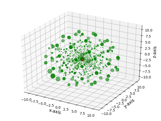
The package comes with functions to visualize meshes. The function plot_mesh_3d() will open an interactive 3d plot with grid points colored in green, and the atoms colored in their respective CPK color. The grid points can be scaled by their respective weights.
>>> from var_mesh import plot_mesh_3d
>>> mesh = dft.Grids(mol)
>>> mesh.level = 0
>>> mesh.build()
>>> plot_mesh_3d(mesh, weight=True)
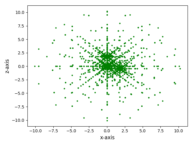
The grid can be projected to a given plane, and the grid points can be scaled by a given integer.
>>> from var_mesh import plot_mesh_2d
>>> plot_mesh_2d(mesh, weight=5, plane='xz')
The script for this example can be downloaded here.
3.4. Precise option
The fine grid search is enabled by default but can be disabled with the parameter precise. Disabling this option will result in a faster grid generation process, but the resulting grid may be larger.
>>> from timeit import default_timer
>>> start = default_timer()
... mesh = var_mesh(mf.grids, thres=1e-8, precise=False)
... end = default_timer()
... print('Time spent = %f seconds' % (end - start))
... print('Mesh points = %d' % len(mesh.coords))
Atom grids = {'H': (60, 434), 'O': (90, 590)}
Time spent = 1.228876 seconds
Mesh points = 60828
This can be compared to the output when the parameter precise is set to True
>>> start = default_timer()
... mesh = var_mesh(mf.grids, thres=1e-8, precise=True)
... end = default_timer()
... print('Time spent = %f seconds' % (end - start))
... print('Mesh points = %d' % len(mesh.coords))
Atom grids = {'H': (50, 302), 'O': (90, 590)}
Time spent = 3.657851 seconds
Mesh points = 48500
The script for this example can be downloaded here.
3.5. Mode option
The mode parameter will change the format of the final grid output. These outputs can be reused in the respective codes. Currently, the mode 'pyscf', 'erkale', and 'gamess' are supported (case-insensitive).
>>> mesh = dft.Grids(mol)
>>> print('mode=PySCF:')
>>> var_mesh(mesh, mode='pyscf')
mode=PySCF:
PySCF grid: atom_grid = {'H': (30, 110), 'O': (60, 302)}
If the code does not support different grids for different atom types, the precise option has no effect. If it is turned on, a warning will be generated.
>>> print('mode=ERKALE:')
>>> var_mesh(mesh, precise=True, mode='erkale')
mode=ERKALE:

WARN: The precise parameter has no effect when using 'gamess' mode.

ERKALE grid: DFTGrid 60 -302
Also, only the largest atom grid will be used in an optimization step. Thus, the atom grids will differ from the default 'pyscf' mode and will be the same for every atom type.
>>> print('mode=GAMESS:')
>>> mesh = var_mesh(mesh, precise=False, mode='gamess')
mode=GAMESS:
GAMESS grid: $dft nrad=60 nleb=302 $end
>>> print('GAMESS grid: %s' % mesh.atom_grid)
GAMESS atom grids: {'H': (60, 302), 'O': (60, 302)}
The script for this example can be downloaded here.
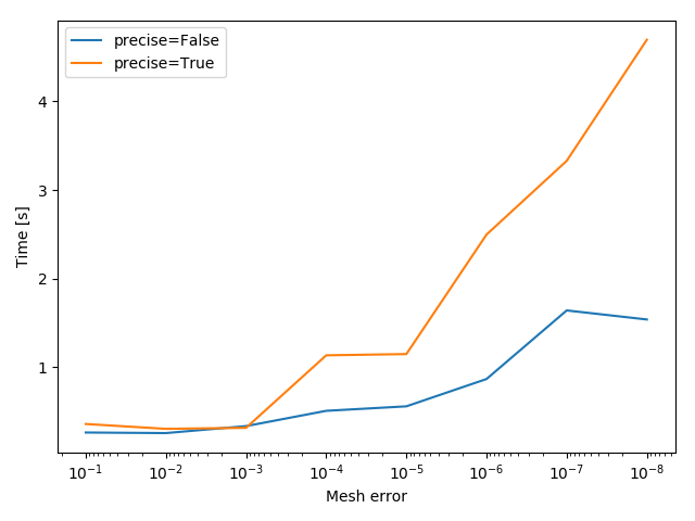
3.6. Mesh time
A more sophisticated way to show the time difference would be to time both options for a set of different thresholds.
>>> import numpy as np
>>> errors = 10.0**(np.arange(-1, -9, -1))
>>> print(errors)
[1.e-01 1.e-02 1.e-03 1.e-04 1.e-05 1.e-06 1.e-07 1.e-08]
A code to time the different options can look like the following
>>> times_false = []
>>> times_true = []
>>> for i in range(len(errors)): \
...     t1 = default_timer() \
...     mesh = var_mesh(mesh, thres=errors[i], precise=False) \
...     t2 = default_timer() \
...     mesh = var_mesh(mesh, thres=errors[i], precise=True) \
...     t3 = default_timer() \
...     times_false.append(t2 - t1) \
...     times_true.append(t3 - t2)
These result can be plotted afterwards.
>>> import matplotlib.pyplot as plt
>>> plt.plot(errors, times_false, label='precise=False')
>>> plt.plot(errors, times_true, label='precise=True')
>>> plt.xlabel('Mesh error')
>>> plt.ylabel('Time [s]')
>>> plt.xscale('log')
>>> plt.gca().invert_xaxis()
>>> plt.legend()
>>> plt.show()
The script for this example can be downloaded here.
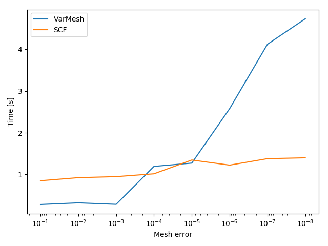
3.7. Calculation time
Another interesting aspect might be the grid generation time in relation to the DFT calculation time.
>>> mf = dft.RKS(mol)
>>> mf.verbose = 0
>>> mf.grids.verbose = 0
>>> time_mesh = []
>>> time_scf = []
>>> for i in range(len(errors)): \
...     t1 = default_timer() \
...     mf.grids = var_mesh(mf.grids, thres=errors[i], precise=True) \
...     t2 = default_timer() \
...     mf.kernel() \
...     t3 = default_timer() \
...     time_mesh.append(t2 - t1) \
...     time_scf.append(t3 - t2)
These result can be plotted as well.
>>> plt.plot(errors, time_mesh, label='VarMesh')
>>> plt.plot(errors, time_scf, label='SCF')
>>> plt.xlabel('Mesh error')
>>> plt.ylabel('Time [s]')
>>> plt.xscale('log')
>>> plt.gca().invert_xaxis()
>>> plt.legend()
>>> plt.show()
The script for this example can be downloaded here.
3.8. PyFLOSIC example
This package can be used with the pyflosic package, too. Since pyflosic only supports Python 3, this example can not be executed with Python 2. The package ase is required as well.
>>> from ase.io import read
>>> from flosic_os import ase2pyscf, xyz_to_nuclei_fod
>>> from flosic_scf import FLOSIC
H2.xyz>>> molecule = read('H2.xyz')
>>> geo, nuclei, fod1, fod2, included = xyz_to_nuclei_fod(molecule)
>>> mol = gto.M(atom=ase2pyscf(nuclei), basis='6-311++Gss', spin=0, charge=0)
>>> sic_object = FLOSIC(mol, xc='lda,pw', fod1=fod1, fod2=fod2, ham_sic='HOO')
>>> sic_object.max_cycle = 300
>>> sic_object.conv_tol = 1e-7
By default a grid level of 3 will be used. Here we compare the mesh size before and after the optimization.
>>> mesh_size = len(sic_object.calc_uks.grids.coords)
>>> print('Mesh size before: %d' % mesh_size)
Mesh size before: 28186
>>> sic_object.calc_uks.grids = var_mesh(sic_object.calc_uks.grids)
>>> print('Mesh size after: %d' % len(sic_object.calc_uks.grids.coords))
Mesh size after: 6600
Finally, start the FLO-SIC calculation.
>>> sic_object.kernel()
ESIC = -0.045866
ESIC = -0.045129
ESIC = -0.045133
ESIC = -0.045130
ESIC = -0.045129
ESIC = -0.045129
ESIC = -0.045129
ESIC = -0.045129
ESIC = -0.045129
ESIC = -0.045129
ESIC = -0.045129
ESIC = -0.045129
ESIC = -0.045129
converged SCF energy = -1.18118690828491  <S^2> = 6.6613381e-16  2S+1 = 1
The script for this example can be downloaded here.